30 Apr 2018
Below is my implementation of the adam optimizer with learning rate multipliers, implemented and tried together with TensorFlow backend.
from keras.legacy import interfaces
import keras.backend as K
from keras.optimizers import Optimizer

class Adam_lr_mult(Optimizer):
    """Adam optimizer.
    Adam optimizer, with learning rate multipliers built on Keras implementation
    # Arguments
        lr: float >= 0. Learning rate.
        beta_1: float, 0 < beta < 1. Generally close to 1.
        beta_2: float, 0 < beta < 1. Generally close to 1.
        epsilon: float >= 0. Fuzz factor. If `None`, defaults to `K.epsilon()`.
        decay: float >= 0. Learning rate decay over each update.
        amsgrad: boolean. Whether to apply the AMSGrad variant of this
            algorithm from the paper "On the Convergence of Adam and
            Beyond".
    # References
        - [Adam - A Method for Stochastic Optimization](http://arxiv.org/abs/1412.6980v8)
        - [On the Convergence of Adam and Beyond](https://openreview.net/forum?id=ryQu7f-RZ)

    AUTHOR: Erik Brorson
    """

    def __init__(self, lr=0.001, beta_1=0.9, beta_2=0.999,
                 epsilon=None, decay=0., amsgrad=False,
                 multipliers=None, debug_verbose=False,**kwargs):
        super(Adam_lr_mult, self).__init__(**kwargs)
        with K.name_scope(self.__class__.__name__):
            self.iterations = K.variable(0, dtype='int64', name='iterations')
            self.lr = K.variable(lr, name='lr')
            self.beta_1 = K.variable(beta_1, name='beta_1')
            self.beta_2 = K.variable(beta_2, name='beta_2')
            self.decay = K.variable(decay, name='decay')
        if epsilon is None:
            epsilon = K.epsilon()
        self.epsilon = epsilon
        self.initial_decay = decay
        self.amsgrad = amsgrad
        self.multipliers = multipliers
        self.debug_verbose = debug_verbose

    @interfaces.legacy_get_updates_support
    def get_updates(self, loss, params):
        grads = self.get_gradients(loss, params)
        self.updates = [K.update_add(self.iterations, 1)]

        lr = self.lr
        if self.initial_decay > 0:
            lr *= (1. / (1. + self.decay * K.cast(self.iterations,
                                                  K.dtype(self.decay))))

        t = K.cast(self.iterations, K.floatx()) + 1
        lr_t = lr * (K.sqrt(1. - K.pow(self.beta_2, t)) /
                     (1. - K.pow(self.beta_1, t)))

        ms = [K.zeros(K.int_shape(p), dtype=K.dtype(p)) for p in params]
        vs = [K.zeros(K.int_shape(p), dtype=K.dtype(p)) for p in params]
        if self.amsgrad:
            vhats = [K.zeros(K.int_shape(p), dtype=K.dtype(p)) for p in params]
        else:
            vhats = [K.zeros(1) for _ in params]
        self.weights = [self.iterations] + ms + vs + vhats

        for p, g, m, v, vhat in zip(params, grads, ms, vs, vhats):

            # Learning rate multipliers
            if self.multipliers:
                multiplier = [mult for mult in self.multipliers if mult in p.name]
            else:
                multiplier = None
            if multiplier:
                new_lr_t = lr_t * self.multipliers[multiplier[0]]
                if self.debug_verbose:
                    print('Setting {} to learning rate {}'.format(multiplier[0], new_lr_t))
                    print(K.get_value(new_lr_t))
            else:
                new_lr_t = lr_t
                if self.debug_verbose:
                    print('No change in learning rate {}'.format(p.name))
                    print(K.get_value(new_lr_t))
            m_t = (self.beta_1 * m) + (1. - self.beta_1) * g
            v_t = (self.beta_2 * v) + (1. - self.beta_2) * K.square(g)
            if self.amsgrad:
                vhat_t = K.maximum(vhat, v_t)
                p_t = p - new_lr_t * m_t / (K.sqrt(vhat_t) + self.epsilon)
                self.updates.append(K.update(vhat, vhat_t))
            else:
                p_t = p - new_lr_t * m_t / (K.sqrt(v_t) + self.epsilon)

            self.updates.append(K.update(m, m_t))
            self.updates.append(K.update(v, v_t))
            new_p = p_t

            # Apply constraints.
            if getattr(p, 'constraint', None) is not None:
                new_p = p.constraint(new_p)

            self.updates.append(K.update(p, new_p))
        return self.updates

    def get_config(self):
        config = {'lr': float(K.get_value(self.lr)),
                  'beta_1': float(K.get_value(self.beta_1)),
                  'beta_2': float(K.get_value(self.beta_2)),
                  'decay': float(K.get_value(self.decay)),
                  'epsilon': self.epsilon,
                  'amsgrad': self.amsgrad,
                  'multipliers':self.multipliers}
        base_config = super(Adam_lr_mult, self).get_config()
        return dict(list(base_config.items()) + list(config.items()))
In addition to the normal parameters, the optimizer takes the multiplier argument which is a dictionary. It works like follows: Imagine if we have a network with three layers with names layer_1, layer_2, and layer_3. This would then be:
learning_rate_multipliers = {}
learning_rate_multipliers['layer_1'] = 1
learning_rate_multipliers['layer_2'] = 0.5
learning_rate_multipliers['layer_3'] = 0.1
We then create the optimizer like so:
adam_with_lr_multipliers = Adam_lr_mult(multipliers=learning_rate_multipliers)
Which can be used to train a model.
24 Mar 2018
import keras as k
import numpy as np
import pandas as pd
import tensorflow as tf
Experimenting with sparse cross entropy
I have a problem to fit a sequence-sequence model using the sparse cross entropy loss. It is not training fast enough compared to the normal categorical_cross_entropy. I want to see if I can reproduce this issue.
First we create some dummy data
X = np.array([[1,2,3,4,5], [0,1,2,3,4]]).reshape(2,5)
Y = k.utils.to_categorical(X, 6)
Then we define a basic model which ties the weight from the embedding in the output layer
input = k.layers.Input((None, ))
embedding = k.layers.Embedding(6, 10)
lstm_1 = k.layers.LSTM(10, return_sequences=True)
embedding_input = embedding(input)
lstm_1 = lstm_1(embedding_input)
lambda_layer = k.layers.Lambda(lambda x: k.backend.dot(
        x, k.backend.transpose(embedding.embeddings)))
lambd = lambda_layer(lstm_1)
softmax = k.layers.Activation('softmax')(lambd)
arg_max = k.layers.Lambda(lambda x: k.backend.argmax(x, axis=2))(softmax)
model = k.Model(inputs = input, outputs=lambd)
model_sparse = k.Model(inputs = input, outputs=lambd)
Now we want to compile our model using, first the categorical_crossentropy loss to make sure everything runs fine. We want to make sure we are tracking accuracy as well, we need to implement this function ourselves…
def sparse_loss(target, output):
    # Reshape into (batch_size, sequence_length)
    output_shape = output.get_shape()
    targets = tf.cast(tf.reshape(target, [-1]), 'int64')
    logits = tf.reshape(output, [-1, int(output_shape[-1])])
    print('logits ',logits.get_shape())
    res = tf.nn.sparse_softmax_cross_entropy_with_logits(
        labels=targets,
        logits=logits)
    if len(output_shape) >= 3:
        # if our output includes timestep dimension
        # or spatial dimensions we need to reshape
        res = tf.reduce_sum(res)
        return(res)
    else:
        return(res)
def normal_loss(y_true, y_pred):
    loss = tf.nn.sparse_softmax_cross_entropy_with_logits(labels=y_true, logits=y_pred)
    return(tf.reduce_sum(loss))
model.compile(k.optimizers.SGD(lr=1), normal_loss,
             target_tensors=[tf.placeholder(dtype='int32', shape=(None, None))])
model_sparse.compile(k.optimizers.SGD(lr=1), sparse_loss,
                    target_tensors=[tf.placeholder(dtype='int32', shape=(None, None))])
# model_sparse.compile(k.optimizers.SGD(lr=1), sparse_loss)
print(model.evaluate(X, X))
print(model_sparse.evaluate(X, X))
2/2 [==============================] - 0s 48ms/step
17.917783737182617
2/2 [==============================] - 0s 113ms/step
17.917783737182617
model_sparse.fit(X,X, epochs=10)
Epoch 1/10
2/2 [==============================] - 1s 388ms/step - loss: 17.9178
Epoch 2/10
2/2 [==============================] - 0s 4ms/step - loss: 17.9026
Epoch 3/10
2/2 [==============================] - 0s 7ms/step - loss: 17.8617
Epoch 4/10
2/2 [==============================] - 0s 5ms/step - loss: 17.7170
Epoch 5/10
2/2 [==============================] - 0s 8ms/step - loss: 17.2932
Epoch 6/10
2/2 [==============================] - 0s 8ms/step - loss: 16.3683
Epoch 7/10
2/2 [==============================] - 0s 9ms/step - loss: 14.0281
Epoch 8/10
2/2 [==============================] - 0s 5ms/step - loss: 10.6938
Epoch 9/10
2/2 [==============================] - 0s 6ms/step - loss: 10.7706
Epoch 10/10
2/2 [==============================] - 0s 10ms/step - loss: 16.4204


<keras.callbacks.History at 0x11590c1d0>
model.fit(X, X, epochs=10)
Epoch 1/10
2/2 [==============================] - 0s 248ms/step - loss: 15.0457
Epoch 2/10
2/2 [==============================] - 0s 6ms/step - loss: 11.0899
Epoch 3/10
2/2 [==============================] - 0s 7ms/step - loss: 6.4245
Epoch 4/10
2/2 [==============================] - 0s 8ms/step - loss: 4.6941
Epoch 5/10
2/2 [==============================] - 0s 7ms/step - loss: 3.1935
Epoch 6/10
2/2 [==============================] - 0s 7ms/step - loss: 2.8392
Epoch 7/10
2/2 [==============================] - 0s 8ms/step - loss: 1.1097
Epoch 8/10
2/2 [==============================] - 0s 8ms/step - loss: 0.6671
Epoch 9/10
2/2 [==============================] - 0s 9ms/step - loss: 0.5167
Epoch 10/10
2/2 [==============================] - 0s 12ms/step - loss: 0.4167


<keras.callbacks.History at 0x116a14ba8>
05 Nov 2017
Let’s play a little game. Given four words, pick the one that is the least like the other. For example, given the word Queen, King, Prince, and Cleaner. Which word would you pick? Personally, I would say that Cleaner is the odd one as the other three are related to royalty and the fourth isn’t. I think most people – at least those who share some of my cultural biases – would agree with me. Now imagine if we could ask a computer the same question. Would it pick the same word? Let’s return to this query later.
Let’s stop for a moment and think about what it actually means to participate in the aforementioned game. We take four words as input and output one word which we think is the most unlike the other. We evaluate each word in relation to the others and might take things as spelling, connotations and semantics into consideration. The words are evaluated in the context of the others. We might think of a king and think of royalty, castles, and power. We know that a king is married to a queen and that their son will be called prince. The choice of word in this example is trivial.
Let’s return to the idea of a computer that is able to perform this task. I built small program in Python that achieves this. I will not go into any technical details in this blog post but figured that it might be interesting to list a few of the choices my program made. Feel free to compare, would you make the same decisions as the AI?
| Example |
Words |
Pick of the AI |
| 1. |
Addition, Christmas, Integral, Pythagoras |
Christmas |
| 2. |
Am, I, Is, The |
The |
| 3. |
Bicycle, Cinnamon, Pump, Wheel |
Cinnamon |
| 4. |
Companionship, Friendship, Hate, Love |
Companionship |
| 5. |
Five, Seven, Thousand, Three |
Thousand |
I made a game out of this which can be played in the console where you can see if you can guess which word the AI picked. Below is a link to the GitHub project. The file called create_new_pairs.py contains the code for the discussed model.
Link to the GitHub project
01 Oct 2017
In this post we continue to discuss the vectorisation of tweets. The technique that I discuss in this post will be used in an upcoming post where we will try it out on the data from the Kaggle competitions used in the earlier post.
Motivation
In the earlier post we quantified the tweets as bag of word-vectors. We are now going to look at a more sophisticated way of vectorising tweets based on word2vec vectors. These vectors are described in a paper by Tomas Mikolov, Kai Chen, Greg Corrado, and Jeffrey Dean. Each word is represented by an n-dimensional vector in such a way that the distance between two words that are semantically similar is shorter that two words that are semantically less similar. For example, if we had two word pairs (King, Man) and (King, Woman) we want the distance between the words in the first pair to be smaller than the distance between the words in the second pair.
These word embeddings are learned using a neural network that predicts the probability of one word being close to another word in a text. We will cover these models and how to implement them in Tensorflow in a future blog post.
The rest of this post is structured as follows. We start off by looking at the word embeddings we will use in the later tweet2vec processing and through a couple of examples get an intuition of how they work.
The pretrained Google word2vec embeddings
In order to learn word2vec embeddings you need to have a very big corpus of texts and substantial computational resources. Lucky for us, there are easier ways to get the embeddings without paying hundreds of dollars in EC2 costs. We are going to use a pretrained model released by Google that can be downloaded here. How to use this model is adequately described in this blogpost.
To get to the word embedding vectors we need to put the whole model in memory. We are going to use the gensim package. The code belows imports the model into memory.
import gensim

# import the word2vec model to memory
word2vec_model = gensim.models.KeyedVectors.load_word2vec_format(
    '/Volumes/PICS/pyProject/GoogleNews-vectors-negative300.bin.gz',
    binary = True)
The file containing the word2vec model is 1.5 gb, so make sure you have enough memory available. It takes a few minutes to load.
Let’s take it for a spin
Let’s run some code. We want to find whether or not the similarities behave in such a way as described earlier. We want to see if the similarity between the words man and king is bigger than the similarity between woman and king. We also want to see the dimensions of the word vectors.
# first, grab the vector
king = word2vec_model.wv['king']

# print its dimensions
print('The dimension of one word vector is: ' + str(king.shape))

# check the similarity between king and man and compare it
#   to king and woman
man_king_sim   = word2vec_model.wv.similarity('king', 'man')
woman_king_sim = word2vec_model.wv.similarity('king', 'woman')

print('The similarity between the words \'king\' and \'man\' is ' + str(man_king_sim))
print('The similarity between the words \'king\' and \'woman\' is ' + str(woman_king_sim))
The dimension of one word vector is: (300,)
The similarity between the words 'king' and 'man' is 0.229426704576
The similarity between the words 'king' and 'woman' is 0.12847973557
As we see, it is as we predicted. And we also see that our are of length 300, neat! Next: let’s see how we can use these word vectors to go from word2vec to tweet2vec!
Let’s say that we want to use these vectors for something more useful, for example as inputs to a machine learning model? If our data would be tweets, we would need to find a way to represent full sentences as vectors an not only individual words. There are a bunch of different ways to do this, for example we could just take the element wise mean of the vectors in a sentence. We find a naive implementation of this idea below in the function text2vec.
# some dependencies
import numpy as np
import nltk
from nltk.corpus import stopwords
from nltk.tokenize import word_tokenize
import string

punctuation_traslator = str.maketrans('', '', string.punctuation)
stop_words = set(stopwords.words('english'))


def text2vec(text):
    """
    takes a string as input, returns a vector representation
        calculated by taking the mean of the individual word
        embedding vectors.

    ARGS:
    - text

    Returns:
    - A vector representation of the
    """
    text = text.lower()
    text = text.translate(punctuation_traslator)
    text = nltk.word_tokenize(text)
    filtered_sentence = [w for w in text if not w in stop_words]
    i = 1
    vector_representation = np.zeros((1,300))

    for word in filtered_sentence:
        try:
            vector_representation = vector_representation + word2vec_model.wv[word]
            i = i + 1
        except KeyError:
            i = i
    vector_representation = np.divide(vector_representation, i)
    return(vector_representation)
Let’s see what the vector for the sentence I really want to have some cheese looks like.
# first, we store our sentence in a variable
sentence = 'I really want to have some cheese'

# second, we process our vector representation of the sentence
sentence_in_vector_form = text2vec(sentence)

# now, let's print the first 10 elements of the vector
print(sentence_in_vector_form[0:10])
[[-0.01306152  0.04898071  0.01190186  0.18371582 -0.03271484
0.05787659
   0.10913086 -0.07702637  0.01344299  0.03594971 -0.04655457
-0.11230469
  -0.03070068 -0.07617188 -0.16723633  0.1484375  ...]]
25 Sep 2017
This is a short demonstration of the text processing capabilities of R as well as a very basic example of how one can go from text based data to a simple model. It showcases a way of turning human-readable tweets into numerical data.
The data used in this example comes from the Kaggle competition called Partly Sunny with a Chance of Hastags. The dataset was contributed by the data library CrowdFlower and contains labelled tweets about the weather. I will use the training set provided for this competition and aims to build a model that predicts the negative sentiment of each tweet.
Let’s get computing!
Since we are going to do some data munging to get everything nice and orderly we use the tidyverse, readr to read data from the harddrive efficiently and tibble to store it in memory. GGplot2 creates nice visualizations. The real work horse in this example is the fantastic tm, or text mining package which supplies us with the option of transforming the tweets into numerical data. At last we are going build a LASSO regression model and keep the modelling data stored in a sparse matrix format that only keeps the non zero elements of the matrix.
library(tidyverse)
library(tm)
library(Matrix)
library(glmnet)
We read in the data but only keep two variables, the tweet itself and the column s2 that corresponds to the negative sentiment of the tweet. We also store the s2 values as a matrix for the later modelling.
Below we see some examples of negative tweets
#Read data from csv-file
tweetData <- read_csv(file = "train.csv",
                      col_types = cols_only(tweet = col_character(),
                                            s2 = col_double()))

#Save negative sentiment in a vector that is to be predicted in later modelling
s2 <- as.matrix(tweetData$s2)

#Print some tweets ordered by negative sentiment
arrange(tweetData, desc(s2))
## # A tibble: 77,946 × 2
##                                                                          tweet
##                                                                          <chr>
## 1  I'm gonna do big things today: running during shit weather and writing my e
## 2                                                @mention cold cloudy rainy :(
## 3                                                             too hot out here
## 4  I'm SO happy we're getting this race in today but goodness... This humidity
## 5             My client said its not cold outside girl puhlezz its bur is shyt
## 6            Dang only 72degrees today, where is all the warm spring weather??
## 7  @mention I do have to agree with you, My lawn is getting about 12" tall, It
## 8  RT @mention: Sick of wearin a hoodie one day n the next day wearin flip flo
## 9  I hate when a shoot is cancelled & rescheduled due to weather then an hour
## 10                                        My boxer is not liking this weather!
## # ... with 77,936 more rows, and 1 more variables: s2 <dbl>
We already get a few ideas on what might be good signals of negative sentiment in the tweets. For example, the first example contains a swear word, shit, which makes the tweet negative. Our goal today is to find a list of such words. The approach is pretty simple, we want to create a simple vectorisation of the tweets and then use those vectors as inputs to a machine learning model.
In this case we are satisfied with just treating the tweets as bag of words. That is, each position in the vector corresponds to a certain word and its value to the number of times the word occurs in the tweet. If we had two tweets that said:
- The weather is bad
- Ugh, bad bad weather
We could construct the vectors, v_1, v_2 where v = (n_the, n_\weather, n_\is, n_\bad, n_\ugh) as:
- v_1 = (1,1,1,1,0)
- v_2 = (0,1,0,2,1)
We also need to process the tweets abit before we go ahead and create the vectors. We want to remove punctuation and stop words since these does not carry any interesting information about the sentiment. Below we see the code to perform this in R. First we create a data representation called corpus. We want to make sure that we are only working with a plain text source, so we transform our corpus using the tm_map function. This function is a wrapper to work with the corpus files in the tm package. The first argument it takes is the corpus and the rest are functions with additional arguments.
After the punctuations and the stopwords are removed we also stem the document, this means that we will represent similar words that differ only in their endings as one word. The stemmed versions of terrible and terribly would be terribl. We then create the tweet vectors using the DocumentTermMatrix function.
At last we pass the document term matrix through the removeSpareTerms function which removes words that are very rare in the corpus. In our example with the tweets above we could for example remove the words the, Ugh and is because they are only present in a single tweet or observation.
#Create a corpus representation of the tweets
corp <- Corpus(VectorSource(tweetData$tweet))
corp <- tm_map(corp, PlainTextDocument)
# Removes punctiation
corp <- tm_map(corp, removePunctuation)
# Remove stopwords
corp <- tm_map(corp, removeWords, stopwords("en"))
# Stem words in the tweets
corp <- tm_map(corp, stemDocument, language = "english")
# Create the matrix and remove unuseful terms

dtm <- DocumentTermMatrix(corp)
dtm <- removeSparseTerms(dtm, 0.999)
So finally, we have our data processed and ready. Now, since our goal is to create a list of words that are associated with tweets about bad weather, we use a simple model that is easy to interpret. We use a regularized version of the linear regression which combines L1 and L2 regularization, also called elastic net logistic regression.
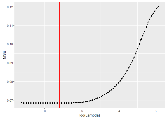
We prepare our data using the built in spare.model.matrix function. To find the appropriate amount of regularization we use a cross-validation approach to find it. The plot below shows the error plotted against different values of the lambda parameter. We choose to use the value that minimizes the error.
data <- cbind(s2, data.frame(as.matrix(dtm)))
# Create a sparse model matrix to be used as input in the model
mat <- sparse.model.matrix(s2~. ,data)

# Use cross-validation to optimize the regularization
model <- cv.glmnet(y = s2, x = mat, alpha = 0.5)
At last we refit our model to the data using the tuned lambda value. The model we are using is linear so each word has its own beta parameter. The value of the parameter can be intepreted as the marginal increase of expected negativity score if the word is in the tweet. So a higher parameter value indicates that the word has a negative sentiment. Below we see the list of the 10 words that has the highest parameter estimates.
finalModel <- glmnet(y = s2, x = mat, alpha = 0.5,
                     lambda = model$lambda.min)
coef <- tibble(variable = row.names(finalModel$beta),
               beta = as.numeric(finalModel$beta))
arrange(coef, desc(beta))
## # A tibble: 1,077 × 2
##    variable      beta
##       <chr>     <dbl>
## 1    crappi 0.5117718
## 2    shitti 0.4595968
## 3   horribl 0.4562549
## 4   depress 0.4292953
## 5      suck 0.4175831
## 6     nasti 0.4157189
## 7    dreari 0.4069617
## 8     miser 0.3783830
## 9      crap 0.3428576
## 10  terribl 0.3324477
## # ... with 1,067 more rows
As we see in the model, the words are stemmed as discussed before. It is obvious that our model managed to find negative words such as crappi, shitti or depress.